9.4 Dynamic path analysis

The term dynamic path analysis was coined by Odd Aalen and coworkers (Aalen, Borgan, and Gjessing 2008). It is an extension, by explicitly introducing time, of path analysis described by Wright (1921).

The inclusion of time in the model implies that there are one path analysis at each time point, see Figure 9.3.

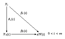
FIGURE 9.3: Dynamic path analysis

\(X_2\) is an intermediate covariate, while \(X_1\) is measured at baseline (\(t =0\)). \(dN(t)\) is the number of events at \(t\).

The structural equations \[\begin{equation*} \begin{split} dN(t) &= \bigl(\beta_0(t) + \beta_1(t) X_1 + \beta_2(t) X_2(t)\bigr)dt + dM(t) \\ X_2(t) &= \theta_0(t) + \theta_1(t) X_1 + \epsilon(t) \end{split} \end{equation*}\] are estimated by ordinary least squares (linear regression) at each \(t\) with \(dN(t) > 0\).

Then the second equation is inserted in the first:

\[\begin{equation*} dN(t) = \{\beta_0(t) + \beta_2(t) \theta_0(t) + \bigl(\beta_1(t) + \theta_1(t) \beta_2(t)\bigr) X_1 + \beta_2(t) \epsilon(t)\}dt + dM(t) \end{equation*}\]

and the total treatment effect is \(\bigl(\beta_1(t) + \theta_1(t)\beta_2(t)\bigr)dt\), so it can be split into two parts according to \[\begin{equation*} \begin{split} \text{total effect} &= \text{direct effect} + \text{ indirect effect} \\ &= \beta_1(t)dt + \theta_1(t)\beta_2(t)dt \end{split} \end{equation*}\] Some book-keeping is necessary in order to write an R function for this dynamic model. Of great help is the function risksets in eha; it keeps track of the composition of the riskset over time, which is exactly what is needed for implementing the dynamic path analysis.

Estimation: Standard least squares at each \(t, \; 0 < t < \infty\) (in principle).

References

Aalen, O. O., Ø. Borgan, and H. K. Gjessing. 2008. Survival and Event History Analysis: A Process Point of View. New York: Springer.

Wright, S. 1921. “Correlation and Causation.” Journal of Agricultural Research 20: 557–85.