9.2 Causal inference

According to Aalen, Borgan, and Gjessing (2008), there are three major schools in statistical causality, (i) graphical models, (ii) predictive causality, and (iii) counterfactual causality. They also introduce a new concept, dynamic path analysis, which can be seen as a merging of (i) and (ii), with the addition that time is explicitly entering the models.

9.2.1 Graphical models

Graphical models have a long history, emanating from Wright (1921) who introduced path analysis. The idea was to show by writing diagrams how variables influence one another. Graphical models has had a revival during the last decades with very active research, see Pearl (2000) and Lauritzen (1996). A major drawback, for event history analysis purposes, is, according to Aalen, Borgan, and Gjessing (2008), that time is not explicitly taken into account. Their idea is that causality evolves in time, that is, a cause must precede an effect.

9.2.2 Predictive causality

The concept of predictive causality is based on stochastic processes, and that a cause must precede an effect in time. This may seem obvious, but very often you do not see it clearly stated. This leads sometimes to confusion, for instance to questions like “What is the cause, and what is the effect?”.

One early example is Granger causality (Granger 1969) in time series analysis. Another early example with more relevance in event history analysis is the concept of local dependence. It was introduced by Tore Schweder (Schweder 1970).

Local dependency is exemplified in Figure 9.1.

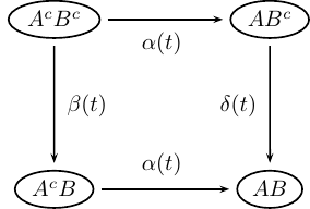
FIGURE 9.1: Local dependence.

Here \(A\) and \(B\) are events, and the superscript (\(c\)) indicates their complements, i.e. they have not (yet) occurred if superscripted. This model is used in the matched data example concerning infant and maternal mortality in a nineteenth century environment later in this chapter. There \(A\) stands for mother dead and \(B\) means infant dead. The mother and her new-born (alive) infant is followed from the birth to the death of the infant (but at most a one-year follow-up). During this follow-up both mother and infant are observed and the eventual death of the mother is reported. The question is whether mother’s death influences the survival chances of the infant (it does!).

In Figure 9.1: If \(\beta(t) \ne \delta(t)\), then \(B\) is locally dependent on \(A\), but \(A\) is locally independent on \(B\): The vertical transition intensities are different, which means that the intensity of \(B\) happening is influenced by \(A\) happening or not. On the other hand, the horizontal transitions are equal, meaning that the intensity of \(A\) happening is not influenced by \(B\) happening or not. In our example this means that mother’s death influences the survival chances of the infant, but mother’s survival chances are unaffected by the eventual death of her infant (maybe not probable in the real world).

9.2.3 Counterfactuals

In situations, where interest lies in estimating a treatment effect (in a wide sense), the idea of counterfactual outcomes is an essential ingredient in the causal inference theory advocated by Rubin (1974) and Robins (1986). A good introduction to the field is given by Hernán and Robins (2020).

Suppose we have a sample of individuals, some treated and some not treated, and we wish to estimate a marginal (in contrast to conditional) treatment effect in the sample at hand. If the sample is the result of randomization, that is, individuals are randomly allocated to treatment or not treatment (placebo), then there are in principle no problems. If, on the other hand, the sample is self-allocated to treatment or placebo (an observational study), then the risk of confounders destroying the analysis is overwhelming. A confounder is a variable that is correlated both with treatment and effect, eventually causing biased effect estimates.

The theory of counterfactuals tries to solve this dilemma by allowing each individual to be its own control. More precisely, for each individual, two hypothetical outcomes are defined; the outcome if treated and the outcome if not treated. Let us call them \(Y_1\) and \(Y_0\), respectively. They are counterfactual (counter to fact), because none of them can be observed. However, since an individual cannot be both treated and untreated, in the real data, each individual has exactly one observed outcome \(Y\). If the individual was treated, then \(Y = Y_0\), otherwise \(Y = Y_1\). The individual treatment effect is \(Y_1 - Y_0\), but this quantity is not possible to observe, so how to proceed?

The Rubin school fixes balance in the data by matching, while the Robins school advocates inverse probability weighting . Both these methods are possible to apply to event history research problems (Hernán, Brumback, and Robins 2002; Hernán et al. 2005), but unfortunately there is few, if any, publicly available R packages for performing these kinds of analyzes, partly with the exception of matching, of which an example is given later in this chapter. However, with the programming power of R, it is fairly straightforward to write own functions for specific problems. This is however out of the scope of this presentation.

The whole theory based on counterfactuals relies on the assumption that there are no unmeasured confounders. Unfortunately, this assumption is completely un-testable, and even worse, it never holds in practice.

References

Aalen, O. O., Ø. Borgan, and H. K. Gjessing. 2008. Survival and Event History Analysis: A Process Point of View. New York: Springer.

Granger, C. W. J. 1969. “Investigating Causal Relations by Econometric Models and Cross-Spectral Methods.” Econometrica 37: 424–38.

Hernán, M. A., B. Brumback, and J. M. Robins. 2002. “Estimating the Causal Effect of Zidovudine on Cd4 Count with a Marginal Structural Modelfor Repeated Measures.” Statistics in Medicine 21: 1689–1709.

Hernán, M. A., S. R. Cole, J. B. Margolick, M. H. Cohen, and J. M. Robins. 2005. “Structural Accelerated Failure Time Models for Survival Analysis in Studies with Time-Varying Treatments.” Pharmacoepidemiology and Drug Safety 14: 477–91.

Hernán, M. A., and J. M. Robins. 2020. Causal Inference: What If. London: Chapman & Hall/CRC.

Lauritzen, S. L. 1996. Graphical Models. Oxford Statistical Science Series No. 17. Oxford, UK: Oxford University Press.

Pearl, J. 2000. Causality: Models, Reasoning and Inference. New York: Cambridge University Press.

Robins, J. M. 1986. “A New Approach to Causal Inference in Mortality Studies with a Sustained Exposure Period—Application to Control of the Healthy Worker Survivor Effect.” Mathematical Modeling 7: 1393–1512.

Rubin, D. B. 1974. “Estimating Causal Effects of Treatments in Randomized and Non-Randomized Studies.” Journal of Educational Psycology 66: 688–701.

Schweder, T. 1970. “Composable Markov Processes.” Journal of Applied Probability 7: 400–410.

Wright, S. 1921. “Correlation and Causation.” Journal of Agricultural Research 20: 557–85.