Chapter 11 Competing Risks Models
Classical competing risks models will be discussed, as well as their modern interpretations. The basic problem is that we want to consider more than one type of event, but where exactly one will occur. For instance, consider death in different causes.
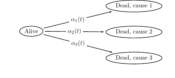
FIGURE 11.1: Competing risks: Causes of death.
The first problem is: How can the intensities \[\begin{equation*} \bigl(\alpha_1(t), \alpha_2(t), \alpha_3(t)\bigr), \quad t > 0 \end{equation*}\] be nonparametrically estimated? It turns out that this is quite simple. The trick is to take one cause at at time and estimate its intensity as if the rest of the causes (events) are censorings. The real problem starts when we want to have these intensities turned into probabilities.
11.1 Some Mathematics
First we need some strict definitions, so that the correct questions are asked, and the correct answers are obtained.
The cause-specific cumulative hazard functions are \[\begin{equation*} \Gamma_k(t) = \int_0^t \alpha_k(s) ds, \quad t > 0, \quad k = 1, 2, 3. \end{equation*}\] The total mortality is \[\begin{equation*} \begin{split} \lambda(t) &= \sum_{k=1}^3 \alpha_k(t)\quad t > 0 \\ \Lambda(t) &= \sum_{k=1}^3 \Gamma_k(t), \quad t > 0 \end{split} \end{equation*}\] and total survival is \[\begin{equation*} S(t) = \exp\left\{-\Lambda(t)\right\} \end{equation*}\] So far, this is not controversial. But asking for a “cause-specific survivor function” is.
11.2 Estimation
The quantities \(\Gamma_k, \; k = 1, 2, 3\), \(\Lambda\), and \(S\) can be estimated in the usual way. \(\Gamma_1\), the is estimated by regarding all other causes (2 and 3) as censorings. The total survivor function \(S\) is estimated by the method of Kaplan-Meier, regarding all causes as the same cause (just death).
Is it meaningful to estimate (calculate) \(S_k(t) = \exp\left\{-\Gamma_k(t)\right\}, \; k = 1, 2, 3\)? The answer is “No.” The reason is that it is difficult to define what these probabilities mean in the presence of other causes of death. For instance, what would happen if one cause was eradicated?
11.3 Meaningful Probabilities
It is meaningful to estimate (and calculate)
\[\begin{equation*}
P_k(t) = \int_0^t S(s) \alpha_k(s) ds,\quad t > 0,\quad k = 1, 2, 3,
\end{equation*}\]
the probability to die from cause \(k\) before time \(t\).
Note that
\[\begin{equation*}
S(t) + P_1(t) + P_2(t) + P_3(t) = 1 \texttt{ for all $t > 0$}.
\end{equation*}\]
Now, estimation is straightforward with the following estimators:
\[\begin{equation*}
\hat{P}_k(t) = \sum_{i:t_i \le t} \hat{S}(t_i-)\frac{d_i^{(k)}}{n_i}
\end{equation*}\]
See the function comp at the end of this chapter for how to write code for
this estimation.
11.4 Regression
It is also possible to include covariates in the estimating procedure.
\[\begin{equation*}
P_k(t) = 1 - \exp\left\{-\Gamma_k(t)\exp\left(X\beta^{(k)}\right)\right\}, \quad
t > 0, \quad k = 1, 2, 3.
\end{equation*}\]
These equations are estimated separately. In R, this can be done with the package
cmprsk (Fine and Gray 1999; B. Gray 2020).
People born in Skellefteå in northern Sweden around the year 1800 are followed over time from 15 years of age to out-migration or death. Right censoring occurs for those who are still present on January 1, 1870. At exit the cause is noted, see Figure 11.2.

FIGURE 11.2: Mortality and emigration, Skellefteå, 1800–1870.
The first rows of the data are shown in Table ??.
The variable event is coded as shown in Table ??.
The code for the function comp is displayed at the end of this
chapter. It is not necessary to understand before reading on. It may be
useful as a template if you want to analyze competing risks.

FIGURE 11.3: Cause-specific exit probabilities; mortality and migration from Skellefteå.
However, a simpler alternative is to use the function survfit in the survival package, see Figure 11.4, where the analysis is performed separately for men and women.

FIGURE 11.4: Mortality and migration, Skellefteå 1820–1935.
Note that the survival is not explicitly shown in Figure 11.4, and the reason is that it is redundant, the sum of all probabilities at any fixed age in Figure 11.3 is equal to one (an individual must be in one and only one state at each age; note that “survival” really means “survived and still present in Skellefteå,” the state all start in at age 15).
And with covariates and cmprsk; the syntax to get it done is a little
bit nonstandard. Here moving to other parish in Sweden is analyzed
(failcode = 2). See Table ??.
library(cmprsk)
xx <- model.matrix(~ sex + soc + illeg, zz)[, -1]
systim <- system.time(fit <- crr(zz$exit, zz$event, xx, failcode = 2))
summary(fit)
The system time for this call is 1 hour and 15 minutes.
The function crr is very slow with large data sets. Therefore I have refrained
from calculating likelihood ratio p-values, so the ones in Table ??
are the Wald ones. However, it seems as if all covariates have a high explanatory value,
and we note that females move within Sweden more than men, and so do white collar people
compared to to the rest. Farmers are the most stationary ones, not surprisingly.
Maybe more surprising is the fact that people born outside marriage are more prone to migrate,
at least within Sweden.
Note that this is not Cox regression (but close!). The corresponding Cox regression result is shown in Table 11.1.
fit <- coxreg(Surv(enter, exit, event == "Sweden") ~ sex + soc +
                  illeg, data = zz)
cap <- "Cox regression, moved to other parish in Sweden."
lab <- "withcox11"
fit.out(fit, caption = cap, label = lab)| Covariate | level | W_mean | Coef | HR | SE | LR_p |
|---|---|---|---|---|---|---|
| sex | 0.0000 | |||||
| male | 0.509 | 0 | 1 | |||
| female | 0.491 | 0.4503 | 1.5688 | 0.0223 | ||
| soc | 0.0000 | |||||
| farming | 0.655 | 0 | 1 | |||
| official | 0.021 | 1.1722 | 3.2290 | 0.0505 | ||
| business | 0.012 | 1.0233 | 2.7823 | 0.0678 | ||
| worker | 0.312 | 0.5895 | 1.8031 | 0.0229 | ||
| illeg | 0.0000 | |||||
| FALSE | 0.959 | 0 | 1 | |||
| TRUE | 0.041 | 0.2218 | 1.2483 | 0.0477 | ||
| Max Log | Likelihood | -89750.3 |
As can be seen from Table 11.1, the same conclusions can be drawn with an ordinary Cox regression as with the competing risks approach, in this case, that is.
What about migrating to countries outside Scandinavia? The same covariates, but
stratified on sex, see Table 11.2 and Figure 11.5.
| Covariate | level | W_mean | Coef | HR | SE | LR_p |
|---|---|---|---|---|---|---|
| soc | 0.0003 | |||||
| farming | 0.655 | 0 | 1 | |||
| official | 0.021 | -0.0493 | 0.9519 | 0.1742 | ||
| business | 0.012 | 0.0633 | 1.0654 | 0.2064 | ||
| worker | 0.312 | 0.2176 | 1.2431 | 0.0499 | ||
| illeg | 0.2237 | |||||
| FALSE | 0.959 | 0 | 1 | |||
| TRUE | 0.041 | -0.1488 | 0.8618 | 0.1251 | ||
| Max Log | Likelihood | -18146.8 |
Here illegitimacy does not mean much, but it is the workers that dominate migration in this case.

FIGURE 11.5: Cumulative hazard functions for males and females, migration outside Scandinavia.
Males end up with a double cumulative intensity of migrating, but the females start earlier.
11.5 R Code for Competing Risks
The code that produced Figure 11.3 is shown here.
function (enter, exit, event, start.age = 0)
{
    par(las = 1)
    if (is.factor(event)) {
        event <- as.numeric(event) - 1
    }
    n <- max(event)
    rs.tot <- risksets(Surv(enter, exit, event > 0.5))
    haz.tot <- rs.tot$n.events/rs.tot$size
    n.t <- length(haz.tot) + 1
    S <- numeric(n.t)
    S[1] <- 1
    for (i in 2:n.t) S[i] <- S[i - 1] * (1 - haz.tot[i - 1])
    haz <- matrix(0, nrow = n, ncol = length(haz.tot))
    P <- matrix(0, nrow = n, ncol = length(haz.tot) + 1)
    for (row in 1:n) {
        rs <- risksets(Surv(enter, exit, event == row))
        haz.row <- rs$n.events/rs$size
        cols <- which(rs.tot$risktimes %in% rs$risktimes)
        haz[row, cols] <- haz.row
        P[row, 2:NCOL(P)] <- cumsum(S[1:(n.t - 1)] * haz[row,
            ])
    }
    plot(c(start.age, rs.tot$risktimes), S, ylim = c(0, 1), xlim = c(start.age,
        max(rs.tot$risktimes)), xlab = "Age", type = "s", ylab = "Probability")
    for (i in 1:n) lines(c(start.age, rs.tot$risktimes), P[i,
        ], lty = i + 1, type = "s")
    legend("left", lty = 1:(n + 1), legend = c("Survival", "Dead",
        "Other parish", "Scandinavia", "Off Scandinavia"), cex = 0.8)
}
<bytecode: 0x56229645c368>